A lab that aspires to do advanced electronic research or product development must have one or more oscilloscopes and spectrum analyzers. Despite their obvious similarities, the two are totally different instruments. The oscilloscope functions in both time and frequency domains, the latter by means of its math/FFT (Fast Fourier transform) capability. The spectrum analyzer, in contrast, does not do time domain work. But it has extraordinary bandwidth for displaying a signal in the frequency domain, a wealth of features that permit in-depth analysis, and controls that provide immense insight and understanding of the waveform and circuitry under investigation.
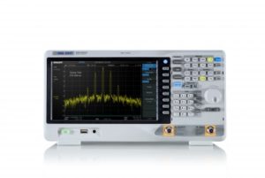
Siglent SSA3032X Spectrum Analyzer
You might wonder how instrument developers provide these capabilities without running the cost into the stratosphere. One design strategy employs a technology that has been around almost a hundred years. The superheterodyne radio receiver was invented in 1918 by Edwin Armstrong, and it was a significant advance over crystal detectors and simple triode vacuum tube radios. Today it is used almost universally in radio and TV receivers and in radar installations.
The idea behind the superheterodyne receiver is rather simple. The modulated RF signal as received at the antenna, tuned to the desired frequency and amplified in the front end, is mixed with a signal produced by a local oscillator so a lower and more manageable beat signal at an intermediate frequency (IF), which is still modulated, can undergo some serious amplification prior to extraction of the audio signal. The audio is further amplified so it can drive a speaker.
Spectrum analyzers fall into two categories, the swept or superheterodyne spectrum analyzer and the FFT instrument, which does not make use of the superheterodyne principle.
The FFT spectrum analyzer is more costly than the swept type when the comparison is made in terms of bandwidth. However, where cost is not the decisive issue, the FFT-type spectrum analyzer can measure phase and can capture transient events more effectively. This is a capability where, given bandwidth constraints, the oscilloscope with FFT ability can fill the need.
In a swept spectrum analyzer, the locally generated frequency provided by the internal oscillator, in addition to reducing the signal to an IF level, also produces the required sweep of the display scan. Accordingly, the location of the point in the display at any given moment corresponds both to the frequency of the local oscillator and thus to that of the signal at the instrument’s input.
Pressing a button on the oscilloscope front panel instantly converts the time domain representation of a waveform into an equivalent frequency domain representation. The theoretical basis for this equivalence was laid out by Joseph Fourier (1768-1830), an ardent supporter of Bonaparte Napoleon, who investigated heat conduction in solids. What is surprising is that thermal propagation through a solid body takes the form of waves or oscillations in the manner of sound traveling through air or electromagnetic energy moving through a vacuum.
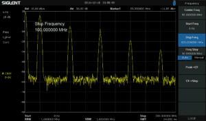
Square wave from the Siglent AWG shown on the Siglent spectrum analyzer. Note powerful harmonics.
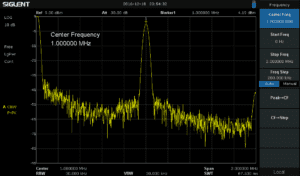
Sine wave from the Siglent AWG shown in Siglent spectrum analyzer.
Fourier conducted a thorough analysis of these and other waveforms arising in nature. He described a constellation of relationships that exist between their time and frequency domain representations.
Fourier’s investigations did not include electrical energy in the form of waves traveling through conductors and higher frequency electromagnetic waves traveling through a vacuum. Nevertheless, his conclusions are absolutely applicable for these phenomena.
Fourier’s conclusions are in his Analytic Theory of Heat, published in 1822. An English-language version is available in Google Books. The lengthy Introduction provides a valuable perspective on the entire work, which is highly technical and math heavy.
Fourier’s important mathematical insight was that any function of a continuous or discontinuous variable can be alternatively expressed as a series of sines of multiples of the variable. This assertion has been amended over the years, but the fundamental relation is valid. And this is precisely how the oscilloscope works, using its math/FFT capability (as well as the spectrum analyzer).
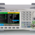
By way of illustration, we’ll connect a Siglent SDG 2122X Arbitrary Waveform Generator first to a Tektronix MDO3104 Oscilloscope and then to a Siglent SSA 3032X Spectrum Analyzer. Using a BNC cable, we connect Output 1 of the Siglent AWG to Analog Channel One in the oscilloscope. We’ll look at two representative waveforms, sine and square wave, in the time domain and in the frequency domain.
Now, staying connected to the Siglent AWG Output 1, we’ll swing the downstream end of the BNC cable to the RF input in the Siglent Spectrum Analyzer. To get a meaningful display in this profound instrument, it is necessary to understand the geometry of its display, specifically in regard to Center Frequency, Start Frequency, Stop Frequency, Span and Frequency Step. With these in mind, we must follow a certain protocol if a signal’s fundamental and harmonics are to be displayed:
1. Power up the Siglent AWG. Check that the Channel 1/Channel 2 button is toggled so as to display Channel One in the AWG. (This is just a thumbnail, not a dynamic trace.)
2. Press Waveforms and the soft key associated with Sine.
3. Press Parameters (or use the touch screen) and using the keypad set the frequency to 10 MHz. Toggle Output 1 so that it is On. This completes the AWG setup.
4. Power up the Siglent SSA 3032 Spectrum Analyzer. Notice that at this point there is not a meaningful display. The trace is a relatively flat noise floor, typical of any frequency domain instrument.
5. Recall that the AWG’s sine wave frequency was set at 10 MHz. Press the top control button labeled Frequency in the spectrum analyzer and using the keypad set the Center Frequency to 50 MHz. Then press Start Frequency and set it to 0 Hz. Press Stop Frequency and set it for 100 MHz. Still no readable display? The answer is to press Auto Tune. Now we should see a 10-MHz sine wave displayed in the frequency domain.
Notice there is a prominent fundamental at 10 MHz with no appreciable harmonics. That is characteristic of a sine wave. All the power appears at a single frequency.
Returning to the Siglent AWG, we press waveforms and change the output to square wave. Again verify that the output frequency and spectrum analyzer frequencies are as before. They may have to be reset.
What appears now is the square wave fundamental plus prominent harmonics. The Y-axis is calibrated in decibels, a logarithmic scale. Power is represented as opposed to volts as in the time domain version. The X-axis, showing frequency, is not marked numerically, but the values of the fundamental and of the powerful whole integer harmonics can be easily ascertained by counting divisions.
We have noted that the large spikes, slightly smaller than the fundamental, representing sine waves (decomposed from the complex square wave), reside at whole integer frequency intervals from the fundamental. But you may want to know the meaning of the huge spike at the left side of the display.
To be accurate, it is not actually part of the signal of interest. It is an outline of the IF filter. As such, it is the same shape as one half of the original signal. Moreover, in a typical spectrum analyzer, as the low- and high-end frequencies are approached, the noise floor will increase in amplitude. Noise peaks dramatically at the low end, producing the rise mentioned above.
As an interesting variation, in the Siglent AWG, set the source at 2 MHz. In the Siglent spectrum analyzer, make the center frequency also 2 MHz and set the span at 2 MHz as well. What is seen now is a far flatter noise floor and the frequency of interest exclusively, without harmonics because the whole integer multiples are outside of the displayed spectrum.
The post Exploring frequencies with a Siglent SSA 3032X spectrum analyzer appeared first on Test & Measurement Tips.