A previous article covered many of the Tektronix MDO3000 Series Oscilloscope menus and front panel controls. Now we bring the survey closer to completion. Rather than memorizing all the details, you can refer to the user manual, connect to the internal or external AFG for sample waveforms, and start pushing buttons. Don’t worry, the oscilloscope won’t explode provided you:
• Observe voltage and current limits at the inputs.
• Comply with CAT limits.
• Scrupulously avoid the basic error of connecting a probe ground return lead to any voltage that floats above and is referenced to the electrical system ground.
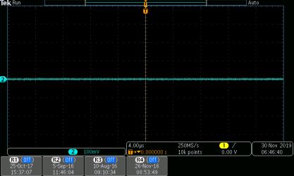
To demonstrate the additional oscilloscope controls and menus, we use two BNC cables to connect Channel One and Channel Two outputs from the AFG to Channel One and Channel two analog inputs in the oscilloscope. When first powered up, the AFG31000 goes to the Home Page. You can navigate through the instrument’s many modes and functions by pressing buttons or by using the touch screen. Most users prefer the quick and easy touch screen, which seems to have no downsides.
In the Home Page, begin by touching Basic. This is the gateway to the library of 12 internal waveforms plus user-created arbitrary waveforms. The two AFG channels are shown in split-screen format. Sine is the default, with other waveforms available in a drop-down menu. Frequency/Period, Phase, Amplitude and Offset can be adjusted. Available modes are Continuous (default), Modulation, Sweep and Burst. All waveform modifications in the AFG are instantly reflected in the two connected oscilloscope channels.
Previously entered Reference waveforms, R1 – R4, are shown in the horizontal Reference menu.
The reference function is used to create and store waveforms. This function permits the user to set up a standard for comparison. The Reference waveforms are nonvolatile and are retained when the oscilloscope is power-cycled. Ten M Reference waveforms, however, are volatile and must be saved to an external drive. To create and store Reference waveforms, press the white R button that sits below the Math button on the front panel. The horizontal Reference menu appears. It consists of a separate listing for each previously created waveform, with date and time. Pressing the associated soft key toggles it on, and it is displayed in the screen above with time stamps for each Reference waveform.
The vertical Reference menu appears to the right. The Reference waveform may be positioned vertically and horizontally, using Multipurpose Knobs a and b. Pressing the appropriate soft key, labels can be inserted and removed. The next soft key displays the sample rate, such as 250 MS/sec, and the record length, such as 10K points. The bottom soft key saves the Reference waveform to external memory or indicates that no drive is available. The internal File Format is .isf and Spreadsheet File Format is .CSV. Press OK Save to complete the operation.
The Search and Marks button and menus are used in conjunction with Wave Inspector to manage long-record-length waveforms and to examine small areas of constrained waveform portions. In Wave Inspector, you can turn the Zoom knob to magnify a waveform horizontally. Turning the Pan knob scrolls through a zoomed waveform. (These are the two large concentric knobs. The small inner knob pans and the large outer knob zooms.)
Pressing the Search button activates the horizontal Search menu. Pressing the soft key associated with the first menu item on the left activates the vertical Search menu. The top soft key toggles Search On and Off. The second soft key clears all marks. The third soft key copies search settings to Trigger. The fourth soft key copies trigger settings to Search. The bottom soft key, labeled More, allows the user to connect Automatic Marks to User Marks, toggle the mark table On and Off, display file details, and save the Mark Table.
Returning to the horizontal Search menu, the second menu item, Search Type, permits the user to turn Multipurpose Knob a to select Edge, Pulse Width, Timeout, Runt, Logic, Setup and Hold, Rise/Fall time and Bus. Each of these Search criteria activates horizontal menus:
Edge activates as Source analog channels one through four, Marks, Reference channels R1 through R4 and digital channels D0 through D15. Source toggles among Rising Slope, Falling Slope or Both. Pulse Width permits the user to set polarity as positive or negative with regard to Search criteria and to set Pulse Width limits and ranges.
To use Marks, first turn on Zoom by pressing the magnifying glass button in the Wave Inspector section. The three Marks buttons sit below the large concentric knobs. Marks can be set and cleared by toggling the Set/Clear button. The Next and Previous arrow buttons move the display among marked locations. Marks can be set automatically using Search criteria. The user can search for and mark regions with unique edges, pulse widths, runts, logic states, rise and fall times, setup and hold and bus types.
Modern digital storage oscilloscopes are capable of displaying electrical signals in the frequency as well as time domain. While lacking some features and having less bandwidth than the considerably more expensive spectrum analyzers, scope-based analyzers are versatile and useful in that they are optimized to display waveforms in the time domain, which is off-limits to the more narrowly focused spectrum analyzer.
We have seen sine and other waveforms displayed in time and frequency domains simultaneously in a mixed domain oscilloscope in the Math mode>FFT.
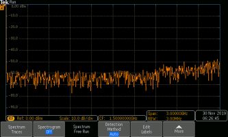
The RF mode lacks time-domain capability but more closely approximates true spectrum analyzer functionality in other respects. There is only one channel, as opposed to two or four analog channels. To see the RF mode in action, we might as well toggle Off the AFG Channel-Two output and swing the BNC cable that is connected to AFG Channel One over to the RF port. (An RF adapter is required.) Then, in the oscilloscope, press the RF button at the right side of the front panel. This turns off all analog channels and displays the sine wave in the frequency domain.
Sine wave in frequency domain
The irregular fluctuating horizontal line, as in Math>FFT, is the instrument’s noise floor. The fundamental is difficult to see because it sits at the extreme left edge of the display. To rectify that situation, as in Math>FFT, we press the Frequency/Span button just below RF. The vertical Frequency and Span menu is activated. Since the sine wave frequency in AFG Channel One is One MHz, we can set the Center Frequency at that value, using Multipurpose Knob a or, better yet, the number pad at the upper right corner of the oscilloscope front panel. Then, make the span two megahertz and you have a highly readable display of the sine wave in the frequency domain.
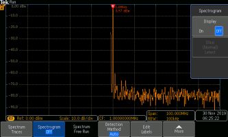
Sine wave fundamental centered in the frequency domain.
Notice that Start and Stop frequencies are automatically adjusted. R to Center is not relevant right now since it applies only to the location of the Reference marker.
In the frequency domain display of the sine wave, all the power is in the fundamental because there are no harmonics visible above the noise floor. To see harmonics, we must shift the AFG output to Square wave. Still, harmonics are not visible because the span is too small. Type in 100 MHz and press Menu Off to see a good array of harmonics generated by the square wave’s fast rise and fall times.
To see an interesting interpretation of harmonics, press RF to go back to the RF menu and press the soft key associated with Spectrogram. In the vertical Spectrogram menu, toggle the display On and press Menu Off to get a look at this different domain. Notice how the display slowly rises from the X-axis to the top of the display.
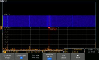
Spectrogram display slowly rises.
You might think the signal is slowly loading, but in reality the Cartesian co-ordinates have once more been redefined. In the Spectrogram, the Y-axis is time rather than amplitude as in the time and frequency domain. The X-axis is frequency. As for amplitude, warmer colors represent higher amplitude and cooler colors represent lower amplitude. To see the passage of time, toggle Spectrogram off and on. Either that, or turn off and on the AFG channel switch.