
The mathematics of humanoid robot walking revolves around balancing dynamics using the center of mass (CoM), kinematic modeling, and trajectory planning. It focuses on the linear inverted pendulum model (LIPM) and the zero-moment point (ZMP) criterion to ensure stability.
It also involves model predictive control (MPC) to control joint trajectories. Plus, divergent components of motion (DCM) are used to predict future CoM behavior to stabilize the robot.
Core concepts are kinematics, the mathematical description of motion. Forward kinematics is used to determine the foot position using joint angles. Inverse kinematics uses matrix algebra to determine the joint angles required when placing a foot at a specific location or set of coordinates.
Degrees of freedom
Degrees of freedom (DoF) refers to the number of ways a joint can move, like rotating or pivoting. A biped humanoid robot requires over 30 DoF for full-body action to enable natural and fluid motions. Human-like walking can be achieved with only 10 to 12 DoF. That can be effective, but can appear “stiff” and unnatural.
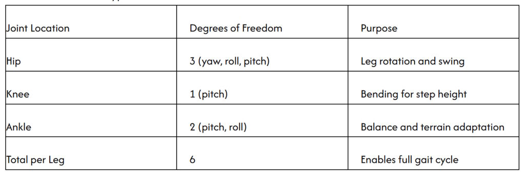
On unlevel surfaces, the ankle joints are especially important. Two DoF, pitch and roll, are required to ensure stability and balanced walking. Without two DoF in the ankles, the robot can be in danger of falling. Basic requirements for simple bipeds include three DoF at the hips (yaw, roll, and pitch), and one DoF (pitch) at the knees, in addition to the two DoF in the ankles (Table 1).
Dynamic matters
There are two phases of walking: the double support phase (DSP), where both feet are on the ground, and the single support phase (SSP), with one foot on the ground. DSP is mathematically modeled by considering constrained contact and requiring smooth transitions for the center of pressure (CoP) and the corresponding CoM. The dynamics of SSP resemble an inverted pendulum, with the swing leg trajectory designed independently using polynomial curves.
Robot walking can be modeled as a tree structure with rigid links using an inverted floating base model where the pelvis is the base and moves relative to an inertial framework. A Jacobian matrix is used to translate the required Cartesian velocities of the feet into angular velocities for the joints.
LIPM simplifies the robot’s complex mass distribution and dynamics into a single point, the CoM, to model and control balance and trajectory. ZPM represents the spot on the ground where the total sum of pitching and rolling moments equals zero. Robot walking shifts the ZPM backward to accelerate the CoM forward.
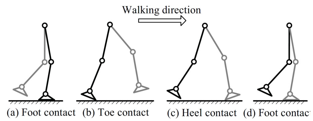
The DCM is used to separate the LIPM dynamics into stable and unstable elements and optimize foot placement and timing. The robot is in the underactuated phase when it has toe or heel contact, and in the fully actuated phase when the robot has full sole contact (Figure 1).
Adding up the maths
The above discussion reviewed some of the common math tools used for humanoid walking. There are numerous frameworks for adding up the maths and training a humanoid to walk. For example, Genetic algorithm optimization tools can be used to tune or “evolve” gait parameters (like step size, speed, and height). In these systems, the ZMP is a key parameter. The algorithm runs thousands of simulated walking sequences, mathematically evaluating the ZMP’s position to ensure it remains well inside the foot’s support polygon before selecting the most stable gait.
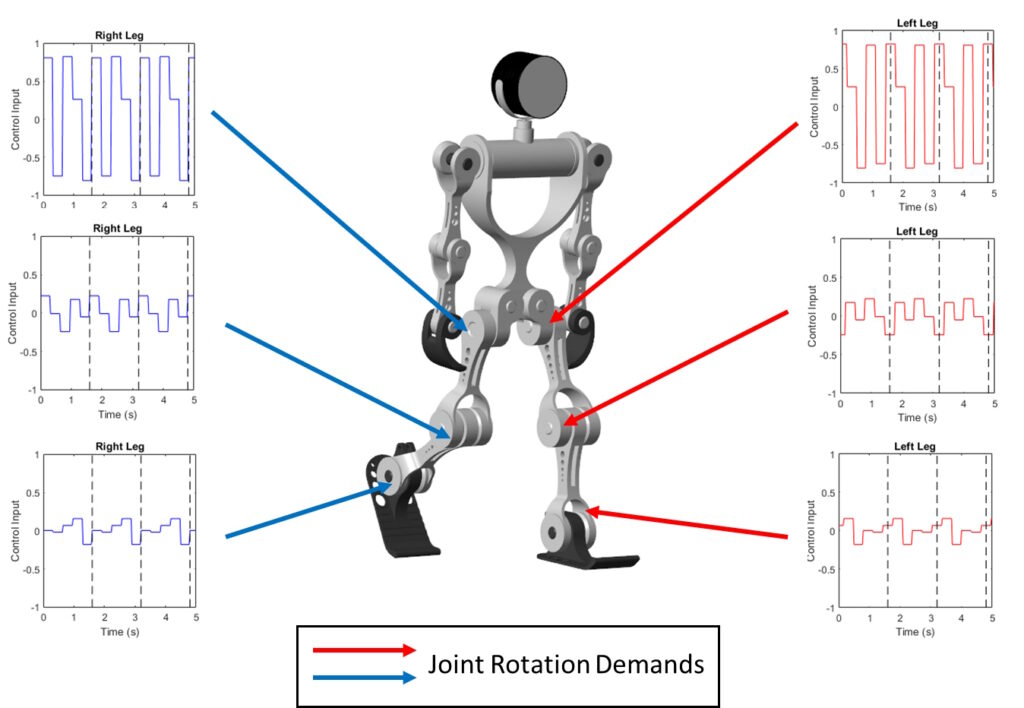
For basic walking, the model determines the repeating pattern for moving the joints. The speed or period of gait is determined by the periodicity of the signals, and that determines the time needed to complete one full step. The control signals for the left and right leg joints are the same, with a relative delay of half the overall gait period (Figure 2).
In some other cases, reinforcement learning (RL) can be used to teach walking to humanoids using trial-and-error-simulations. ZPM can be integrated into the RL framework. Hybrid systems are also used that combine classical physics math with RL. The addition of RL can improve agility and deliver more natural-looking and robust walking compared with genetic algorithms.
Summary
A wide variety of math tools are needed to support balance and enable humanoid robots to walk efficiently. Additional tools enable trajectory and path planning. Finally, like human children, humanoids must learn to walk. Teaching tools for that purpose range from genetic algorithms to advanced RL techniques.
References
An Improved Hierarchical Optimization Framework for Walking Control of Underactuated Humanoid Robots Using Model Predictive Control and Whole Body Planner and Controller, MDPI mathematics
Beyond Wheels: Designing and Building a Walking/Bipedal Robot, KEYi Technology
Gait Generation and Motion Implementation of Humanoid Robots Based on Hierarchical Whole-Body Control, MDPI electronics
Humanoid robot balance control system during backward walking using linear quadratic regulator, IAES International Journal of Robotics and Automation
Precise Calculation of Inverse Kinematics of the Center of Gravity for Bipedal Walking Robots, MDPI applied sciences
Robust Dynamic Walking for Humanoid Robots via Computationally Efficient Footstep Planner and Whole-Body Control, Springer Nature
Walking control of humanoid robots based on improved footstep planner and whole-body coordination controller, Frontiers in Neurorobotics
Walking Pattern Generation Through Step-by-Step Quadratic Programming for Biped Robots, MDPI Biomimetics
Walking Robot Control: From PID to Reinforcement Learning, MathWorks
Related EEWorld Online content
What kinematic equations are important for industrial robots?
What are the types and uses of position sensors?
How is a transformer used in neural networks?
How do ML and AI work in power conversion? part 1
How and where is vapor chamber cooling used?