An overview of filters and their parameters, Part 4: Time and phase issues

Understanding how filters are characterized is the first step in choosing an appropriate topology with suitable specifications.

Thus far, we have focused on filters primarily in terms of their frequency response. However, it is equally legitimate to look at their time-domain and phase-related performance, and in many cases, just as or even more important.

Q: What is the time-domain performance of a filter?

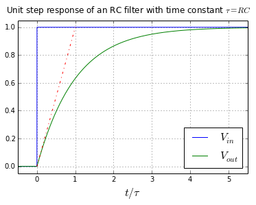
A: In brief, a filter’s response to a signal is not instantaneous. The time-based response indicates, among other things, how long it takes for the filter output to settle to its final value. Most filter designs define this final value as close enough as settling to 1%, 0.1%, or even 0.01% of the final value depending on the application (Figure 1).

Fig 1: The time-domain step response of a filter – here, a basic low-pass RC filter – is not instantaneous but asymptotically approaches the final value. (Image: Embedded Related)

Q: What is this filter time constant which is cited above?

A: In the time domain, for a basic RC low-pass filter, time constant is the time required to charge the capacitor through the resistor, from its initial charge voltage of zero to approximately 63.2% (1 – 1/e) of the value of an applied DC voltage, or to discharge the capacitor through the same resistor to approximately 36.8% (1/e) of its initial charge voltage. The time constant is a good high-level summary of the filter’s time-domain response.

Q: What’s the general relationship between rise and settling time and filter bandwidth?

A: Rise and settling time and 3-dB bandwidth are inversely proportional. For the classic RC low-pass filter, rise time is equal to 0.36.8 divided by 3-dB bandwidth. In general, a wider-bandwidth filter will have a shorter settling time.

Q: What about “Q” and the time domain?

A: In the time domain, Q is an indicator of a filter’s damping characteristics and corresponds to the amount of oscillation in the system’s step response.

Q: Why does settling time matter?

A: If the system is making decisions or taking action based on the output of the filter, it needs to wait until that output has settled before making doing, or else it is using misleading, premature signal values. This applies to all-analog control loops, data acquisition, and digitals systems. A basic RC low-pass filter takes 9.2 R×C time constants for an input step to settle to within 0.01% of its final value.

Q: What’s a scenario for this?

A: Consider a simple data-acquisition system which is measuring a real-world parameter such as flow or pressure from a suitable transducer in the presence of 50/60 Hz ambient noise – a very common scenario. Good engineering practice would put a 50/60 Hz notch filter in the signal path to attenuate that noise. However, as the signal of interest changes, it has to pass through the filter, whose output must settle to the actual value before the output is used. How long to wait – how Many time constants – is a function of the desired accuracy and fidelity.

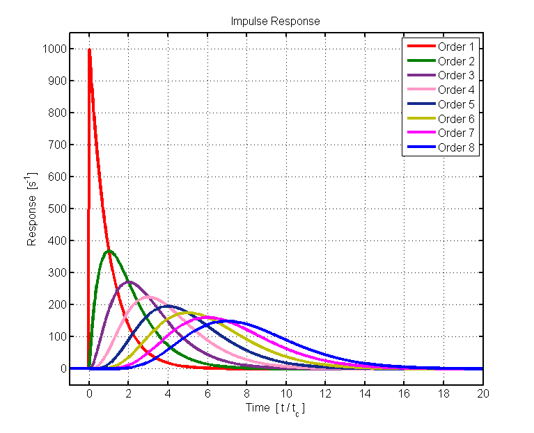
Q: What’s the impulse or step response of a filter?

A: You can characterize the performance of a filter by providing a sweeping sine wave to the filter and measuring the output response versus frequency; this is a standard technique. The sweep rate must be slow enough so that the filter output has time to settle, of course, or the output reading will be erroneous.

An alternative in many cases is to provide a very sharp spike (an impulse) or step wave at the filter input Figure 2. From signal theory and the equivalence of time and frequency domains as linked by the Fourier transform, that impulse or step contains all frequencies. Thus, the impulse response of the filter tells you a great deal about the filter’s performance. In some designs, the time-domain perspective is more useful than the frequency-domain perspective.

Fig 2: The step response of filters of different orders from n=1 to n=8 but with the same time constant (here, 1 msec) clearly shows that the higher the filter order is, the slower the filter response. (Image: Zurich Instruments)

Q: What’s the meaning of quality factor Q in the time domain?

A: In the time domain, the quality factor of a filter characterizes the filter’s damping characteristics, which corresponds to the amount of oscillation in the system’s step response.

Q: So far, there has been no mention of phase in the context of filters – is there a consideration with respect to phase?

A: The phase-related performance of a filter is very important in some cases and not an issue in others. (Keep in mind that phase and frequency are intimately related: frequency in the time-derivative of phase, while phase is the time-integral of frequency.) For applications such as filtering a signal from a sensor, how the filter affect (delays) phase is usually irrelevant.

However, phase-related performance is critical in communications links that phase-modulates the carrier as part of the data encoding. The phase shift introduced by the filter must be analyzed, and the phase performance partially determines the filter choice.

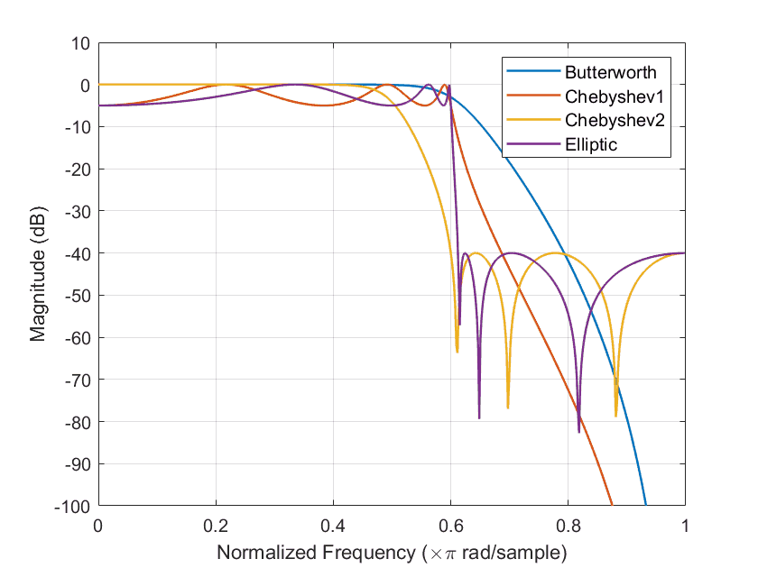
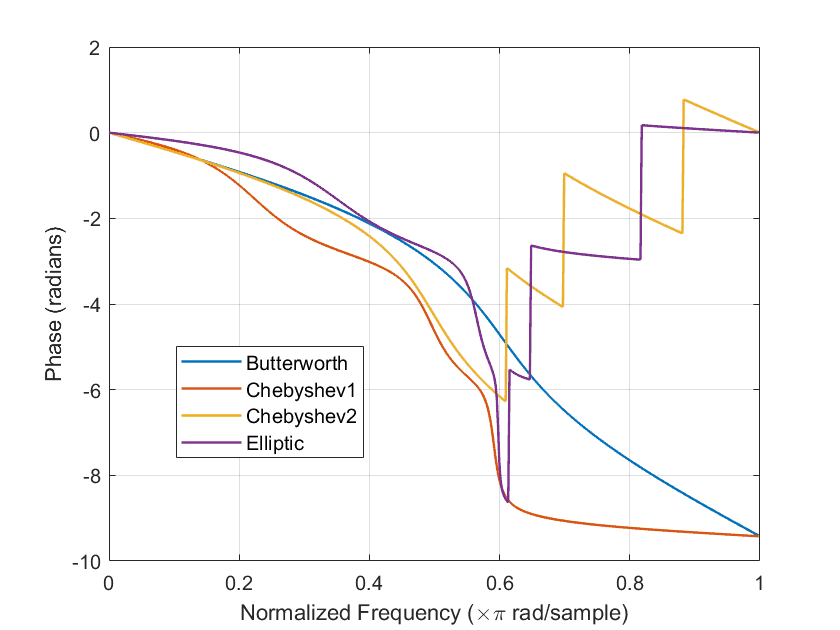
Q: How does phase analysis affect filter analysis?

A: Full filter analysis requires complex numbers and even Bode plots where the input and output signals are characterized both by amplitude versus frequency (Figure 3) and phase shift versus frequency (Figure 4). This makes filter analysis more difficult, but it is doable and very often unnecessary.

Fig 3: The amplitude response versus frequency for four basic filter topologies is important but is not the entire filter-characterization story. (Image: Technobyte.org)

Fig 4: The phase response versus frequency for the same four filter topologies provides the often-important other half of the story. (Image: Technobyte.org)

Q: Are filters ever designed or selected primarily for their phase rather than amplitude performance?

A: Yes, there are cases where meeting phase relationships or adjusting them is as important or perhaps more important than amplitude response. Even filters called “all pass” filters have flat amplitude characteristics across a wide spectrum but user-specified phase response performance in a specific part of the spectrum of interest.

Q: What’s a good way to study filter theory and design?

A: The best way is to start with the basic one-pole RC low-pass filter. This forms the basis for many other filter topologies, considerations, and characterizations. For all analog RLC filters, there are also important issues of the performance sensitivity to initial component tolerance and inevitable temperature drift that add to the analysis complexity.

Q: So far, the discussion has been about filters using discrete RLC components. What else is there?

A: As the filter frequency of operation increases and reaches the hundreds of megahertz and then gigahertz, discrete-components filters become less practical. Their component values get smaller and smaller (down to microhenries and nanofarads and evens smaller), while unavoidable parasitics make the filter hard to model and build. At those frequencies, filters using very different fundamental fabrication techniques such as surface-acoustic wave (SAW) and bulk-acoustic wave (BAW) approaches are used, as well as filters etched in PC boards (stripline and microstrip). These are still analog filters.

There are also discrete-time switched-capacitor (SC) filters based on an array of capacitors which are switched rapidly. SC filters are good at lower-to-mid-range frequencies up to around 1 MHz. One of their major virtues is that they can be fabricated with digital-IC processes and so can be embedded in digital ICs.

Q: What kinds of filter references and tutorial material is available?

A: The good and bad news is that there are a near-infinite number of sources ranging from intuitive to “cookbooks” which require little knowledge, to practical explanations with discussions, and to complex, mathematical-based treatises which examine filter theory and performance. In some ways, it’s too much of a good thing.

Again, most engineers no longer design filters but instead rely on available designs or pre-made (“canned”) filters. Still, given the unrelenting need for filters, their widespread use, and the vital role they have in almost every design, it’s not surprising to see that they receive so much attention and so many resources. That’s why even if a designer is only selecting a filter rather than designing one, it is important to understand their most important parameters to better judge the individual merits and tradeoffs among them, as no filter is ideal in all respects.

Related EE World Content